DeMNISTifying Neural Networks

Abstract

We assume that you are coming from this article right here. If you have not read it yet, we highly recommend to catch up on it before continuing.

What this article is about

MNIST Dataset

In this article we will try to explain the fundamental mechanism behind Neural Networks by discussing and showing off the classification of the very well known MNIST dataset from the National Institute of Standards and Technology. It is a set of handwritten digits from $0$ to $9$ in a $28$ by $28$ grid of pixels in which each pixel has got a value between $0$ and $255$ , representing a tone of gray ( $0$ = black, $255$ = white). In practice, every value is divided by $255$ , so that we only work with percentual values between $0$ and $1$ .

Example of the number nine:

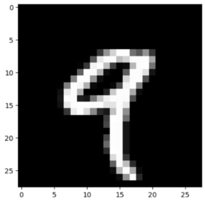
The dataset preserves $60,000$ labeled images to train on and additional $10,000$ labeled images to test the model’s accuracy on unseen data. Our task will be to train a Neural Network with these digits so that it will be able to identify the digits from $0$ to $9$ , of the same format, and yield a most probably correct response on which one it is.

The Neural Network

The development of Neural Networks goes back to the 1940s. In 1943 Warren S. McCulloch and Walter Pitts published their paper “A Logical Calculus of the Ideas Immanent in Nervous Activity”¹ which introduced the idea of a mathematical concept imitating the functionality of biological nerve systems, like the human brain. Furthermore, the concept should be used to solve problems that cannot be described directly in simple rules, but can be worked out by analysing a given set of data and extracting its patterns autonomously. In more direct terms this means that you do not define your mathematical function from the beginning but rather define its outer form and change its inner parameters algorithmically by looking at different data examples. This technique was developed ever since and laid the foundation for the modern Artificial Intelligence (AI) used today. Of course, nowadays, there are a lot of different functions that build on these early developed principles, but a finalized version of the Neural Network exists to this day and will be discussed in the following.

Training Cycle

Neural Networks are trained in three steps:

1. The Forward Pass Firstly, the network looks at one or multiple examples of the data and calculates an output. It may be correct or not. One set of inputs (e. g. the pixels of an image) is called a sample; multiple samples are referred to as a batch. It is indeed possible to process multiple samples, a batch, at once to decrease computing time. At the end of the forward pass the network calculates the loss or cost which measures how different the networks prediction is from the wanted output. The closer the loss is to $0$ , the better the prediction.

2. The Backward Pass Secondly, the network calculates from back to front, the influence of every inner parameter on the prediction using the calculated loss. It figures out which parameters were responsible for it to fail or made the result less precise.

3. Stochastic Gradient Descent Finally, using a method called Stochastic Gradient Descent (SGD), every parameter is changed based on its calculated influence. The goal of this operation is that the same batch would now result in a better prediction. Therefore, if all data samples of the data set follow the same fundamental patterns, the network will slowly learn to make better predictions on the given type of data.

The mathematics behind this training concept will furthermore be discussed.

The Forward Pass

Connecting Neurons Mathematically

This is one of the most common representations of a Neural Network:

In this figure every dot represents a neuron; the connections between the neurons are referred to as weights. Moreover, you may have already noticed the neurons being grouped in layers. The output of the Neural Network is normally calculated step by step by calculating layer after layer from left to right. Every neuron of one layer is connected to every neuron of the previous layer, and therefore receives data from all of the previous neurons. This is why this structure is sometimes called a fully interconnected layer.

\text{Diag. 2}

To sum all this up mathematically, a neuron ${}^Ln_{j}$ of the layer $L$ is a weighted sum of all neurons ${}^{L-1}n_{i}$ of the previous layer $L-1$ . Most importantly, each neuron ${}^Ln_{j}$ has its own weight $w_{i,j}$ for every neuron ${}^{L-1}n_{i}$ , so that it interprets them differently than all the other neurons of the same layer. The input layer $L=0$ is somewhat special because it does not calculate anything. Its neurons are just set to the input, so that each neuron of the layer corresponds to one feature of the input sample, for example, a pixel of an image. Now, we notate every layer as a vector that contains its neurons:

^{L}\vec{n} = \begin{bmatrix} ^{L}n_0 & ^{L}n_1 & \dots & ^{L}n_{m-1} \end{bmatrix}

m \in \mathbb{N}, \text{m is the number of neurons in the layer L}

The input vector of one of the digits of the earlier mentioned MNIST dataset, in which each of the $28 \cdot 28$ pixels $p$ is represented by one tone of gray, would therefore look like this:

\begin{aligned} \vec{in} &= \begin{bmatrix} p_0 & p_1 & \dots & p_{28 \cdot 28 - 1} \end{bmatrix} \\[0.3em] &= \begin{bmatrix} ^0n_0 & {}^0n_1 & \dots & ^0n_{783} \end{bmatrix} \\[0.3em] &= {}^0\vec{n} \end{aligned}

Now, we got an input with which we can begin to calculate our first layer $L=1$ . For every neuron ${}^1n_i$ the following formula applies:

{}^1n_i = \sum_{j=0}^{783} {}^0\vec{n}_j \cdot {}^1\vec{w}_{j}

Here ${}^1\vec{w}$ holds all the connections (the weights) between the neuron ${}^1n_m$ and all the neurons of the first layer ${}^0\vec{n}$ . Of course, ${}^1\vec{w}_0$ corresponds to ${}^1\vec{n}_0$ , ${}^1\vec{w}_1$ corresponds to ${}^1\vec{n}_1$ and so on. The interesting part about this is that you can just rewrite that expression for every neuron as a dot product of the neurons of the previous layer and the respective neuron’s weights:

{}^1n_i = {}^0\vec{n} \cdot {}^1\vec{w} \qquad \dim({}^0\vec{n}) = \dim({}^1\vec{w})

We can take this even further by combining every weight vector of every neuron in a layer in form of a weight matrix ${}^LW$ like this:

{}^LW = \begin{pmatrix} {}^Lw_{0,0} & {}^Lw_{0,1} & \cdots & {}^Lw_{0,m-1}\\ {}^Lw_{1,0} & {}^Lw_{1,1} & \cdots & {}^Lw_{1,m-1}\\ \vdots & \vdots & \ddots & \vdots\\ {}^Lw_{n-1,0} & {}^Lw_{n-1,1} & \cdots & {}^Lw_{n-1,m-1}\\ \end{pmatrix} \qquad \begin{aligned} {}^LW &\in \mathbb{R}^{in, out}\\ n &= \dim({}^{L-1}\vec{n}) \\ m &= \dim({}^{L}\vec{n}) \\ \end{aligned}

Every column now represents all the weights of one neuron of the layer that is being calculated while every row stands for one neuron of the input from the previous layer. If we continue this idea and take the dot product of our input vector ${}^{L-1}\vec{n}$ and the weight matrix ${}^LW$ of the current layer, we get the correct value of each neuron according to the graph (figure 1).

{}^{L-1}\vec{n} \cdot {}^LW \quad=\quad {}^{L}\vec{n}

If we have $n$ neurons in layer $L-1$ and $m$ neurons in layer $L$ , the dimensions of the containers look like this:

{}^{L-1}\vec{n} \in \mathbb{R}^n \qquad {}^{L}W \in \mathbb{R}^{n,m} \qquad {}^{L}\vec{n} \in \mathbb{R}^m \qquad n,m \in \mathbb{N}

This means that for any layer we are mapping $n$ input dimensions to $m$ output dimensions. Then, the explained process is continued with each and every layer of the Neural Network. The amount of layers and neurons in each layer can be defined freely; there is no right or wrong, but some structures, of course, work better for a specific type of data than others do. The only exceptions are the input layer which needs the exact number of neurons of your measured features, and the output layer which also needs to have the right number of neurons. The reason for that will be addressed in one of the following chapters. In practice, this means that every layer owns a weight matrix that indicates all connections to its previous layer. The data example is then encoded as a vector which is furthermore passed forward through the network. Every layer, one after another, multiplies the output vector of the previous layer with its internal weight matrix and passes on its own output vector to the next layer. By the way, the weights are one of the two types of parameters inside the network that change during the training process. They are adjusted so that the network can improve the quality of its predictions.

Adding Bias

In addition to the weights every neuron contains a so called bias that basically is a constant which is added to the weighted sum of the input neurons. This constant ensures that the network is able to shift all inputs and can cover a wider numerical range. Again, we can bundle all biases of one layer $L$ in a vector $\vec{b}$ .

{}^L\vec{b} \in \mathbb{R}^{n} \qquad n \in \mathbb{N}, \quad \text{which is the number of neurons in the layer L}

Now, ${}^L\vec{b}$ is just added to the weighted sum to calculate the layer output:

{}^{L-1}\vec{n} \, \cdot \, {}^LW + {}^L\vec{b} \, = {}^{L}\vec{n}

The bias is trained during training, too. Thus, it is the second parameter which changes during the training process - like the weights.

The Output

As mentioned in the introduction, we are looking for a vector with an element for every class that can possibly be predicted by the network. All these elements together form a probability distribution and the index of the highest value indicates the predicted class. This probability distribution is not important yet, but we already gained the knowledge to understand how the dimensionality of the output comes into place. And it is fairly simple: We just define the last layer of the Neural Network to have one neuron for every class. Mathematically speaking, this means that the last layer $L$ multiplies the output vector of its predecessor $L-1$ with a matrix of the dimensions $\text{inputs x classes}$ and hence mapping the input to the dimension we need. The function $NN$ represents all the calculations done inside the network.

\begin{aligned} NN: \mathbb{R}^f \rightarrow \mathbb{R}^c&, \qquad NN(\vec{in}) = \vec{out}\\ f, c \in \mathbb{N}&, \quad \text{mapping \(f\) inputs to \(c\) outputs} \end{aligned}

Consequently, we can write the Neural Network as a function $NN$ which maps a number of $f$ features in the input sample to a dimension of $c$ which is the number of output classes, by multiplying the input vector $\vec{in}$ with multiple weight matrices $W$ and adding the biases $\vec{b}$ .

But why does this work?

Up to this point we only discussed the mathematical notation of a Neural Network. But why should the concept shown on the graph even be able to find patterns in data and, for example, understand what is shown on an image? Thinking of our current example data of handwritten digits, an ideally set up network could work like this: There is a first input layer followed by a second one. Every neuron in the second layer looks at different neurons of the input. A crucial characteristic of the weights between the neurons is that they can become close to zero during training. As a consequence neurons can learn to under-rate specific neurons of their input or can ignore them completely. Thus, it would be logical for every neuron of a layer to look at a specific area of the image and tell for example whether there is a line or a dot in the top right or the top left corner. If so, the neuron responsible for that would output a high value because in our data white is defined as a high value close to $1$ . The following layer then would continue to group these clusters even more. Does one line extend on another? Do they form a circle? Of course, the exact process depends on the amount of layers and the number of neurons in each of them. But in general this is how you can interpret the passing of information through the layers. Every layer of neurons adds a new layer of abstraction of the image. All pixels are clustered differently again and again until, in the end, the network can make a decision by evaluating all the present features in the image.

The Activation Function

Mathematically speaking, again, the described mechanism can also be interpreted as a regression - which it basically is. We have some datapoints in a very high dimensional space (in our case we have 784 plus additional 10 dimensions to be precise, because of 784 inputs and 10 outputs) and our Neural Network tries to approximate them using a very complex function that is described by means of neurons, weights and biases. But eventhough this function quickly becomes very complex, it has one fundamental problem: It is linear. We neither use any exponential functions, nor logarithms, nor roots, not even an exponent higher than one. As a consequence, the process of regression is limited to linear dependencies. But luckily, there is a simple way to counter this issue. It is called an Activation Function. Basically, we add a non-linear function that is applied to every parameter of the calculated vector after every layer. The function itself does not contain any parameters that change during training, but ensures that the other parameters can have a non-linear influence on the output. The manipulated output of a layer is called an activation and is what is actually passed on to the next layer. A Neural Network $NN$ with one layer and one activation function $a$ can be described like this:

\text{NN}(\vec{in}) = {}^La\left(\vec{in} \cdot {}^{L}W + {}^L\vec{b}\,\right)

Extending this notation, two layers look like this:

\text{NN}(\vec{in}) = {}^La \left({}^{L-1}a\left(\vec{in} \cdot {}^{L-1}W + {}^{L-1}\vec{b}\,\right) \cdot {}^LW + {}^L\vec{b}\,\right) = \vec{out}

And so on.

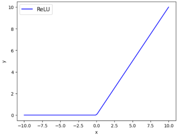
There are a lot of different types of activation functions like the Sigmoid function or Tanh, but one of the most commonly used and easy to calculate functions is the ReLU, which is the short form for Rectified Linear Unit. It just sets all negative values of its input to zero and does not change anything on the positive values. ReLU as a function for some value $x$ has the following form:

\text{ReLU}(x) = \text{max}(0, x) =\begin{cases} 0 & \text{for } x < 0, \\ x & \text{for } x \ge 0. \end{cases} \qquad x \in \mathbb{R}

It results in the following graph and, thus, is not linear:

The Calculation of a Batch

Up to this point we talked about processing only one sample as a vector. But we can actually calculate multiple samples at once as a batch. It is done quite easily by writing multiple samples into a matrix instead of processing them one after another in a vector. Every row becomes a sample while the columns contain the respective features. So, we group multiple input vectors $\vec{in}$ as one input matrix $I$ .

I \in \mathbb{R}^{s, f}, \quad s, f \in \mathbb{N}, \quad \text{for $s$ samples and $f$ features}

{}^LO = {}^La\left({}^{L-1}I \cdot {}^{L}W+ {}^L\vec{b}\,\right)

The activation function ${}^La$ of that layer $L$ is applied to every element of that matrix and every element of the bias vector $\vec{b}$ is added to every value of its respective column in the matrix. The output ${}^LO$ is then passed forward to the successor layer $L+1$ .

The Last Layer

Finally, as soon as the input has gone through all layers except for the last one, this last layer receives a matrix as every layer until then. Even better, this input matrix is processed nearly the same way as before. The layer multiplies the input matrix with its weight matrix to set up the right number of dimensions and furthermore adds a bias vector. The only difference is the activation function $a$ . In our example, in which only one out of the ten classes will be predicted, the output vectors (inside the output matrix ${}^LO$ ) are transformed into a probability distribution using the Softmax function $\sigma$ .

\sigma(X_{i,j})= \frac{e^{X_{i,j}}} {\sum_{k=0}^{dim(X_i)-1}{e^{X_{i,k}}}}

This means that we raise $e$ to the power of every element of the inputed matrix $X$ and divide it by the sum of every element of the same row (also as an exponent of e). We raise $e$ and do not just divide every element by the sum of its row to ensure that we do not get any negative values as a result while not changing the order of the values. An example for three classes could look like this:

X = \begin{pmatrix} -1 & 3 & 2\\ 2 & -2 & 0 \end{pmatrix}

This matrix $X$ contains the so called logits which is the output of two samples of the network before applying the activation function. After applying $\sigma$ to every element transfers to approximately this:

O = \begin{pmatrix} 0.01 & 0.72 & 0.27\\ 0.87 & 0.01 & 0.12 \end{pmatrix}

This output would predict the second class for the first sample with 72% and the first class for the second sample with 87% because these are the highest values in each row.

Notice how the order of the values in each row does not change at all. The highest value stays the highest and the lowest stays the lowest. This means that we would actually not need the softmax function to make a prediction because we can just look at the highest value of the logits and take that as the predicted class. Nevertheless, we make use of the softmax function firstly to make the output more accessible to human beings and secondly to calculate how wrong the prediction of the network was. This is needed to adjust the internal parameters of the network and make it learn.

The Loss Function

Now that we have a predicted probability distribution of an input, we can begin to calculate the accuracy of that prediction. This is done using a Loss or Cost function. As a reminder, we want the neuron of the right class to be close to a value of $1$ and all the other neurons to be close to a value of $0$ . Additionally, our training data is labeled. This means that for every sample we give as a input we already know the right result and, thus, which neuron is the one that needs to be highest. In general, we calculate a batch of samples and compare the network’s prediction with the right solution. The closer the loss is to $0$ the better the prediction; a high loss indicates a bad prediction. As a consequence we want to minimize the loss during training. One of the many Loss functions that does exactly that is the Categorical Cross-Entropy (CCE). It is commonly used for classifications with the softmax function because it is easy to calculate. This is the formula of the CCE:

\text{CCE}(\vec{x}, \vec{t}\,)= -\sum_{i=0}^{\text{dim}(\vec{x})-1}{\vec{t}_i \cdot ln(\vec{x_i})}, \qquad \text{dim}(\vec{x}) = \text{dim}(\vec{t}\,), \qquad i \in \mathbb{N}

The vector $\vec{x}$ is a probability vector of a prediction, like the ones in our output matrix $O$ , and the vector $\vec{t}$ are the targets which are the wanted values of the respective neurons with the same index in the output. A target vector for the classification of the number $4$ would look like this:

\vec{t} = \Big[\, \begin{matrix} 0 & 0 & 0 & 0 & 1 & 0 & 0 & 0 & 0 & 0 \end{matrix} \,\Big]

We will not dive deeper into the reasons for the exact formula of the CCE because, for our scenario, the formula simplifies a lot and it becomes quite clear why it works for us. As you may have noticed, all values of $\vec{x}$ are multiplied by their corresponding target value which is $0$ for most values and $1$ for the targeted class. Consequently, the formula shortens to this:

\text{CCE}(\vec{x}, t) = -ln(\vec{x}_t), \qquad t \in \mathbb{N}

Here, $t$ stands for the index of our target neuron, hence we get the negative natural logarithm of the value of the neuron that represents the targeted class. If we look at the graph for that function, it perfectly matches our needed properties.

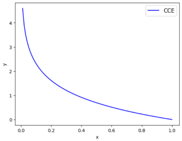
A perfect prediction of the right class with $100\%$ results in a loss of $0$ while the loss skyrockets to infinity when the prediction comes closer to $0\%$ . Additionally, it makes sense that we only look at one value of the output vector because all elements are dependent on each other due to them being part of the same probability distribution. If the target value is high, the average of all the other values becomes low.

But we can go even further and can compress the calculations done even more by combining the softmax $\sigma$ with the CCE. Because we only need one probability value for the loss calculation we do not need to calculate it for every logit. Thus we do the softmax calculation for the target value only and then plug the result into the loss function.

\sigma(X_{i,t})= \frac{e^{X_{i,t}}} {\sum_{k=0}^{dim(X_i)-1}{e^{X_{i,k}}}} \qquad i,t,k \in \mathbb{N}

Above you can see the softmax function for the target logit, indicated by the index $t$ . For a more concise notation we write the exponential sum of the row as an external function $s(\vec{x})$ .

s(\vec{x}) = \sum_{i=0}^{dim(\vec{x})-1}{e^{\vec{x}_{i}}} \qquad \sigma(X_{i,t})= \frac{e^{X_{i,t}}} {s(X_i)} \qquad i,t \in \mathbb{N}

Now we combine the loss with that new version of the softmax function. Additionally, we write the loss as $L_i$ because it represents the loss of the $i$ th sample in the batch.

\begin{aligned} L_i(X_{i,t}) &= -ln\Big(\sigma(X_{i,t})\Big) =-ln\Big(\frac{e^{\scriptstyle X_{i,t}}}{s(X_i)}\Big) \\[0.4em] &=-\Big(ln\Big(e^{\scriptstyle X_{i,t}}\Big)-ln\Big(s(X_i)\Big)\Big)\\[0.4em] &=-\Big(X_{i,t}-ln\Big(s(X_i)\Big)\Big)\\[0.4em] &=ln\Big(s(X_i)\Big) - X_{i,t}\\[0.4em] \end{aligned} \qquad i,t \in \mathbb{N}

Concludingly, we can calculate the loss of a sample by

adding up all its logits and
taking the natural logarithm of that sum and
finally, subtract the value that should be the highest according to our labeled dataset.

For a batch $I$ and the resulting logits $X$ we just take the mean of all the losses $L_i$ of the samples in that batch to calculate the general loss $L_G$ of one forward pass..

L_G=\frac{1}{B}\sum_{i=0}^{B-1}{L_i(O_{i,\vec{t}_i})} \qquad B,i \in \mathbb{N} \qquad \vec{t} \in \mathbb{N}^B

Here, $B$ stands for the number of samples in the batch while the vector $\vec{t}$ holds all the indices of the target classes for each respective sample in the batch.

The Backward Pass

Stochastic Gradient Descent

As we now have a way to measure the models performance on a batch we can continue on how to minimize this performance value step by step. The name of the method used to achieve this is called, as the title of this paragraph suggests, Stochastic Gradient Descent (SGD). The idea of this method is to calculate the influence every parameter has on the output of a function. In other words, we search for the slope of every intrinsic parameter of the Neural Network at a specific point. This specific point at which we want to calculate the slope is always the high dimensional point that we input. After having calculated the slope of all parameters, which is also referred to as a gradient, we subtract that gradient from every parameter and therefore take a step into the opposite direction of the increase. You can imagine that process as a ball that rolls down a high dimensional hill. But it rolls in steps and hence first searches the direction to go up but then continues to roll in the opposite direction. That way, at some point it will reach a local minimum. For our case the following applies: We want to know the mathematical partial derivative of every parameter $p$ in respect to the final Loss $L$ .

\frac{\partial{L}}{\partial{p}}, \quad \text{this is what we want to know for every parameter \(p\) of our network}

Due to all the derivatives of a layer being dependent on its successor’s gradients, the gradients are calculated from back to front of the network. This is why the process is called a backward pass.

The Loss Gradient

Firstly, we need the influence of every output ${}^LO_{i,j}$ of the last layer on the loss. There are two cases between which we have to distinguish: Is the value ${}^LO_{i,j}$ the target of that sample or not. Recalling the simplified formula for the loss $L_i$ from above, it becomes evident why this is the case.

L_i(O_{i,t}) =ln\Big(s(O_i)\Big) - O_{i,t} \qquad s(\vec{x}) = \!\!\!\!\! \sum_{i=0}^{dim(\vec{x})-1}{e^{\vec{x}_{i}}} \qquad i,t \in \mathbb{N}

If $j = t$ the value ${}^LO_{i,j}$ is to be found in the sum of all values in the vector and, additionally, in the subtraction at the end. Consequently, the derivative of any logit ${}^LO_{i,j}$ in the last layer of the network can be notated like this:

\begin{aligned} \frac{\partial{L_i}}{\partial{{}^LO_{i,j}}} &= \frac{\partial}{\partial{{}^LO_{i,j}}}\Big(ln\Big(s(O_i)\Big) - O_{i,t}\Big)\\[0.8em] &= \begin{cases} \frac{\partial}{\partial{{}^LO_{i,j}}}\Big(ln\Big(s(O_i)\Big)- O_{i,t}\Big) & \text{for } j = t\\[0.4em] \frac{\partial}{\partial{{}^LO_{i,j}}}\Big(ln\Big(s(O_i)\Big)\Big) & \text{for } j \ne t\\[0.4em] \end{cases}\\[0.4em] &= \begin{cases} \frac{1}{s(O_i)} \cdot e^{O_{i,j}}-1 & \text{for } j = t\\[0.4em] \frac{1}{s(O_i)} \cdot e^{O_{i,j}} & \text{for } j \ne t\\[0.4em] \end{cases}\\[0.8em] &= \begin{cases} \sigma({}^LO_{i,j})-1 & \text{for } j = t\\[0.4em] \sigma({}^LO_{i,j}) & \text{for } j \ne t\\[0.4em] \end{cases}\\[0.8em] \end{aligned} \qquad i,j,t \in \mathbb{N}

Interestingly, the gradient of the logits ${}^LO$ of the last layer $L$ is just the softmax function of each element ${}^LO_{i,j}$ minus the target value of each logit which is either $1$ or $0$ . The operation $-0$ , of course, is not visible in the last step of the second case. But we still have to multiply every derivative with the constant $\frac{1}{B}$ since we took the mean of the loss of every sample in the batch to create one general loss $L_G$ like this:

L_G=\frac{1}{B}\sum_{i=0}^{B-1}{L(O_{i,\vec{t}_i})} \qquad B,i \in \mathbb{N} \qquad \vec{t} \in \mathbb{N}^B

The corrected derivative for the general loss $L_G$ can furthermore be found with the scalar multiple rule.

\begin{aligned} \frac{\partial{L_G}}{\partial{{}^LO_{i,j}}} &= \frac{1}{B} \cdot \frac{\partial{L_i}}{\partial{{}^LO_{i,j}}}\\[0.4em] &= \begin{cases} \frac{1}{B} \cdot \sigma({}^LO_{i,j})-1 & \text{for } j = t\\[0.4em] \frac{1}{B} \cdot \sigma({}^LO_{i,j}) & \text{for } j \ne t\\ \end{cases} \end{aligned} \qquad i,j,t,B \in \mathbb{N}

If we apply this to every element of our logits we obtain a gradient matrix $G$ with the same dimensions as ${}^LO$ which tells us exactly how much the loss $L_G$ would change if we changed one of the values inside of ${}^LO$ .

The Chain Rule

Before we continue with the calculation of the gradients of the actual parameters which we want to change, let us have a quick look on why it is even necessary to calculate all the derivatives of the output. Our Neural Network can be described as a stack of functions calling each other, thus, the slope of every parameter is dependent on its outer function. This is where the chain rule comes into play. Remember the function $NN$ from earlier that describes a network with two layers. The outer activation function is swapped with the loss $L$ .

\text{NN}(I) = L_G \Big({}^{L-1}a\left(I \cdot {}^{L-1}W + {}^{L-1}\vec{b}\,\right) \cdot {}^LW + {}^L\vec{b}\Big)

If we look at this function, we can trace back how the derivative of ${}^{L-1}W$ in respect to $L_G$ is calculated according to the chain rule.

\frac{\partial L_G}{\partial{}^{L-1}W} = \frac{\partial {}^{L-1}a} {\partial {}^{L-1}W} \cdot \frac{\partial L_G} {\partial {}^{L-1}a}

This works the same way for the bias vector $\vec{b}$ , the input $I$ or even the output ${}^{L-2}O$ of the layer $L-2$ if we had one in this example.

\frac{\partial L_G}{\partial{}^{L-2}O} = \frac{\partial {}^{L-1}a} {\partial {}^{L-2}O} \cdot \frac{\partial L_G} {\partial {}^{L-1}a}

This is why we have to pass the gradient of the input of a layer $L$ to its predecessor $L-1$ , so that it knows how much influence its output ${}^{L-1}O$ has on the loss. We just did the same thing for the last layer $L$ in the previous paragraph where we calculated the gradient for the logits which are the output ${}^{L}O$ of that last layer $L$ .

The Layer Gradients

For every layer there are three gradients to calculate:

the bias gradient $\vec{g}_b$ which indicates the influence of every bias of the layer,
the weight gradient $G_w$ which indicates the influence of every weight of the layer and
the input gradient $G_I$ which indicates the influence of the input that the layer received from the previous layer. This gradient is furthermore given to that predecessor $L-1$ which then does the same calculations for its weights, biases and inputs.

For the following calculations we assume that the layer $L$ is given a gradient $G_X$ which contains the gradient for its output logits ${}^LX$ , by either the activation function between this layer and the successor layer $L+1$ or the loss function.

\text{dim}(G_X)=\text{dim}({}^LX)

1. The Bias Gradient Due to the bias being a constant that is added to the weighted sum of the input neurons, its derivative is zero and, thus, ignores the input ${}^{L-1}O$ and the weight matrix ${}^LW$ completely.

{}^LX = {}^{L-1}O \cdot {}^{L}W+ {}^L\vec{b}

As a reminder, ${}^LX$ represents the output of the layer before the application of the activation function. Rewritten for one sample ${}^{L}X_i$ the formula becomes the following:

{}^LX_{i} = {}^{L-1}O_i \cdot {}^{L}W+ {}^L\vec{b} \qquad i \in \mathbb{N}

This indicates that the derivative of every bias ${}^L\vec{b}_j$ is just $1$ .

\frac{\partial {}^LX_{i,j}}{\partial {}^L\vec{b}_j}=1 \qquad i,j \in \mathbb{N}

To get the influence on the loss $L_G$ , we use the chain rule and multiply the bias’ derivative with the influence of the layer’s result on the loss which is given by its gradient $G_X$ .

\begin{aligned} \frac{\partial L_G}{\partial {}^L\vec{b}_j} &= \frac{\partial {}^LX_{i,j}}{\partial {}^L\vec{b}_j} \cdot \frac{\partial L_G} {\partial {}^LX_{i,j}}\\[0.4em] &= \frac{\partial {}^LX_{i,j}}{\partial {}^L\vec{b}_j} \cdot (G_X)_{i,j}\\[0.4em] &=(G_X)_{i,j} \end{aligned} \qquad i,j \in \mathbb{N}

Therefore, the gradient of one bias is just the gradient of the corresponding neuron’s output, but because we process multiple samples at once we calculate the mean of all the influences that neuron has on every sample $s$ .

(\vec{g_b})_i=\sum_{s=0}^{B-1}{(G_X)_{s,i}} \qquad i,s,B \in \mathbb{N}

A division by the batch size $B$ is not necessary as all gradients in $G_X$ were already divided by $B$ in the calculation of the loss gradient.

2. The Weight Gradient Next, we calculate the gradient matrix $G_W$ of the weights ${}^LW$ . To do so, we first look at the formula for one output neuron $X_{s,i}$ of the sample $s$ :

X_{s,i} =\!\!\!\! \sum_{j=0}^{\text{dim}({}^{L-1}O_s)-1} {{}^{L-1}O_{s,j}\cdot {}^LW_{j,i}} \quad + \, \vec{b}_i \qquad i,j,s \in \mathbb{N}

The partial derivative of one weight ${}^LW_{j,i}$ hence becomes:

\frac{\partial X_{s,i}} {\partial{}^LW_{j,i}} = {}^{L-1}O_{s,j}

Applying the chain rule yields:

\begin{aligned} \frac{\partial L_G} {\partial{}^LW_{j,i}} &= \frac{\partial X_{s,i}} {\partial{}^LW_{j,i}} \cdot \frac{\partial L_G} {\partial {}^LX_{s,i}}\\[0.4em] &= {}^{L-1}O_{s,j} \cdot (G_X)_{s,i} \end{aligned}

This is the gradient for one sample $s$ . But, again, we are looking for a mean over all samples and we can again leave out the division by the batch size $B$ .

\begin{aligned} \frac{\partial L_G} {\partial{}^LW_{j,i}} &= \sum_{s=0}^{B-1}{}^{L-1}O_{s,j} \cdot (G_X)_{s,i} \end{aligned}

The formula above can be concisely written for every weight of ${}^LW$ as a matrix multiplication between the transformed input ${}^{L-1}O$ and the gradient $G_X$ . As a result we receive the weight gradient $G_W$ :

G_W = ({}^{L-1}O)^T \cdot G_X

3. The Input Gradient All that is left to do for the layer is to calculate the influence of the received input ${}^{L-1}O$ . Again, we take the formula for one neuron and take the derivative - this time for the input ${}^{L-1}O_{s,j}$ :

X_{s,i} =\!\!\!\! \sum_{j=0}^{\text{dim}({}^{L-1}O_s)-1} {{}^{L-1}O_{s,j}\cdot {}^LW_{j,i}} \quad + \vec{b}_i \qquad i,j,s \in \mathbb{N}

\frac{\partial X_{s,i}} {\partial{}^{L-1}O_{s,j}} = {}^LW_{j,i}

Again, applying the chain rule provides:

\begin{aligned} \frac{\partial L_G} {\partial{}^{L-1}O_{s,j}} &= \frac{\partial X_{s,i}} {\partial{}^{L-1}O_{s,j}} \cdot \frac{\partial L_G} {\partial {}^LX_{s,i}}\\[0.5em] &= {}^LW_{j,i} \cdot (G_X)_{s,i} \end{aligned}

And again, we sum up everything, but this time over the number of features $f$ , since the input ${}^{L-1}O_{s,j}$ influences every output neuron of the layer:

\frac{\partial L_G} {\partial{}^{L-1}O_{s,j}} = \sum_{i=0}^{f-1} {}^LW_{j,i} \cdot (G_X)_{s,i} \qquad f \in \mathbb{N}

For this expression too, there exists a concise notation as a matrix multiplication:

G_O=G_X \cdot ({}^LW)^T

This gradient is then passes through the activation function to the previous layer $L-1$ which does the same calculations for its parameters.

The Activation Gradient

As there are existing a lot of different activation functions we will not be able to cover all of their partial derivatives. But, at least, we will address the one we used in our example above, the ReLU.

Having the graph above in mind the derivative of the ReLU function can evidently only be $0$ or $1$ , depending on whether the input $x$ is positive or negative. For the function’s input $I$ and its corresponding output $A$ we can write the following partial derivative.

\frac{\partial A_{i,j}}{\partial I_{i,j}} = \begin{cases} 0 & \text{for } I_{i,j} < 0,\\ 1 & \text{for } I_{i,j} \ge 0. \end{cases} \qquad i,j \in \mathbb{N} \qquad \text{dim}(I) = \text{dim}\left(\frac{\partial A}{\partial I}\right)

Then, we apply the respective gradients $G_A$ which we get from the successor layer:

\begin{aligned} (G_I)_{i,j} &= \frac{\partial A_{i,j}}{\partial I_{i,j}} \cdot \frac{\partial L_G}{\partial A_{i,j}}\\[0.4em] &=(G_A)_{i,j}\cdot \begin{cases} 0 & \text{for } I_{i,j} < 0\\ 1 & \text{for } I_{i,j} \ge 0 \end{cases}\\[0.4em] &=\begin{cases} 0 & \text{for } I_{i,j} < 0\\ (G_A)_{i,j} & \text{for } I_{i,j} \ge 0 \end{cases} \end{aligned} \qquad i,j \in \mathbb{N} \qquad \text{dim}(I) = \text{dim}(G_I)

This gets us the gradient $G_I$ of the input $I$ .

Applying The Gradients

Finally, the only thing that is left to do after having calculated every gradient of every parameter of the network is to apply them to the parameters. Since we want to go in the opposite direction than the one the slope is pointing, we subtract the every gradient $g_p$ of the respective parameter $p$ to receive the new parameter $p_{t+1}$ .

p_{t+1} = p - \eta \cdot g_p \qquad t \in \mathbb{N}

Normally, the gradients are scaled by a universal constant $\eta$ called the learning rate. Using this learning rate you can decide how big the steps of adjustment are. A high learning rate results in a fast but imprecise gradient descent while a smaller learning rate goes smaller steps and hence takes longer to reach a local minimum of the loss but will come closer to that minimum. For the best performance, the learning rate usually is adjusted over time during training.

W. S. McCulloch and W. Pitts, “A logical calculus of the ideas immanent in nervous activity,” The bulletin of mathematical biophysics, vol. 5, no. 4, pp. 115–133, Dec. 1943, doi: 10.1007/ BF02478259. ↩︎